Structural Variant Detection using CLC Genomics Workbench

Introduction to the Advanced Structural Variant Detection plugin for the CLC Genomics Workbench

Structural variants affect large regions of the human genome and also play a significant role in gene expression (1, 2). They are typically detected with short Illumina or long PacBio reads, or a combination of both approaches. The new Advanced Structural Variant Detection (ASVD) plugin focuses on the short read approach, and is able to detect structural variants using short Illumina reads from whole genome sequencing (WGS). It supports the detection of the most frequently occurring structural variant types in the human genome such as deletions, duplications, and insertions (1).

Algorithmic steps

The ASVD plugin checks read mappings for evidence of breakpoints using “unaligned end” signatures. “Unaligned end” refers to the end of a read that does not map to the reference sequence. At biological breakpoints, it is expected that multiple reads display unaligned ends, giving rise to a signature. A statistical model evaluates the likelihood of each breakpoint based on the probabilities of supporting reads. Breakpoint signatures and coverage information are next processed together in a series of steps. These include specialized alignment algorithms, copy number variation (CNV) detection, and local de novo assembly. If multiple structural variant calls are based on the set of breakpoints, the optimal calls given the breakpoint evidence are reported as the final set of detected structural variants.

Output

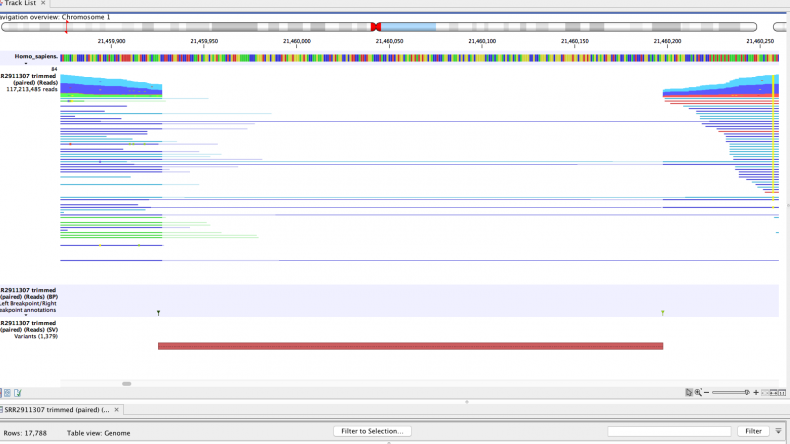
Detected breakpoints and structural variants can be viewed together with the read mappings and the reference sequence. Track tables can then be used to filter and select individual breakpoints and structural variants as shown in the example in Figure 1.

Figure 1. Genome track view of the reference sequence, the read mapping of the sample and a track with the structural variant calls. The table view of the structural variant calls track allows interactive filtering and viewing of the results. An example of “unaligned ends”, i.e. ends of reads that do not match the reference genome, are seen as transparent ends of lines representing reads in the mapping.

Testing

To evaluate the performance of the ASVD plugin, we compared it to Illumina’s Manta. Recent benchmarks against Delly and Lumpy showed that Manta had superior performance (3, 4).

We made use of two recent data sets from Huddleston et al. (5) and Shi et al. (6) to evaluate the ASVD plugin and Manta. Both of these studies used PacBio reads for contig assembly and structural variant detection concerning the GRCh38 reference.

While Shi et al. utilized a diploid genome from an anonymous Chinese individual HX1, Huddleston et al. sequenced two effectively haploid human genomes from hydatidiform moles CHM1 and CHM13 that hence lack allelic variations. Haploid genomes facilitate contig assembly and structural variant detection compared with diploid genomes, and we considered the CHM1 and CHM13 sets the most reliable truth sets available to our knowledge at the time of testing.

We combined the CHM1 and CHM13 sets to produce a diploid truth set, which contained 66.5% more calls than HX1. We believe this difference is mainly caused by the difficulty in detecting structural variants in a diploid genome, where Huddleston et al. showed that they were unable to recover the majority of their heterozygous calls when using an effectively diploid version of CHM1 and CHM13.

CHM1 and CHM13 Illumina reads were sampled to create three different sets of 20x, 40x, and 80x coverages, while the reads available for HX1 provided coverage of 75x. We note that our benchmarking method does not evaluate alternate but equivalent variant representations and that the truth set calls may not always be precise. We, therefore, used an error margin of 50 base pairs when comparing ASVD and Manta calls with structural variants in each truth set (see also special notes for further details regarding benchmarks and data preparation).

Table 1: Benchmark of ASVD and Manta on artificial diploid WGS reads at varying coverage, obtained by sampling form a mix of CHM1 and CHM13 reads in addition to a HX1 comparison. A SV was considered a true positive, if the call was within 50 bp of the truth.

The ASVD plugin and Manta perform comparably across the different sets. Both the ASVD plugin and Manta showed significantly more “false positives” in the HX1 set compared with the Huddleston et al. 20x – 80x sets. We believe this is an artifact of real SVs that are present, but not included in the HX1 truth set.

We assessed the performance separately for short and long structural variants for the typical scenario of 40x coverage Illumina whole genome sequencing. A detailed comparison of results for the Huddleston et al. 40x coverage set in table 2, where we only considered variants of minimum 50 base pairs and applied a cut-off between short and long structural variants at 100 base pairs.

Table 2: Benchmark of ASVD and Manta for short and long structural variants for the 40x coverage Illumina data set. A SV was considered a true positive, if the call was within 50 bp of the truth.

We observed instances where the ASVD plugin and Manta made equivalent calls that appeared correct, but were not present or were represented differently in a truth set. This resulted in lower precision and sensitivity values overall for both tools that is likely to be the case.

Conclusion

These benchmarks suggest that ASVD and Manta have very comparable performances for short SVs and that ASVD performs slightly better than Manta for longer CVs.

Special Notes

• We used BWA 0.7.17-r1194-dirty for aligning reads with Manta 1.5, and our Map Reads to Reference tool in CLC Genomics Workbench 12 with the ASVD plugin. Reads were trimmed using the CLC Trim Reads tool and exported to FASTQ in the case of BWA.
• For benchmarking with the Huddleston et al. truth set, we generated 20x, 40x, and 80x Illumina read sets using CHM1 and CHM13 Illumina reads from the Broad Institute (SRA: ERR1341794 and ERR1341795). Illumina reads for benchmarking with the Shi et al. truth set was accessed from hx1.wglab.org (SRA: SRR2911307).
• Any calls made by the ASVD plugin or Manta in chromatin regions were ignored as these regions are challenging for contig assembly. We only considered truth calls up to 10.000 bp in length, which we based on the PacBio read lengths that were used in the truth set studies.
• Manta raw output contains various flags and representations that should be taken into account to avoid under-representing its performance. As our truth sets only contained deletions and insertions, we split replacements into SNVs and indels and ignored calls with SVTYPE = BND (these are difficult to parse calls that are possible inversions and/or more complicated calls). We also ignored calls that are flagged IMPRECISE and calls that did not have their filter value set to FILTER=PASS. Each of these changes improved Manta’s results compared with the raw output is provided.
• In the case of the Shi et al. HX1 data, the fields in their truth did not appear to be fully documented and so some columns in the set were ignored. We checked the correctness of calls by comparing each inserted/deleted sequence with the length value that was provided.

References

(1) Sudmant, P.H., et al. (2015) An integrated map of structural variation in 2,504 human genomes. Nature, 526
(2) Chiang, C., et al. (2017) The impact of structural variation on human gene expression. Nat. Genet. 49(5):692-699.
(3) Chen, X,., et al. (2016) Manta: rapid detection of structural variants and indels for germline and cancer sequencing applications, Bioinformatics. 32(8):1220-2.
(4) Sedlazeck F J., et al. (2018) Accurate detection of complex structural variations using single-molecule sequencing. Nat. Methods. 15(6):461-468.
(5) Huddleston, J., et al. (2017) Discovery and genotyping of structural variation from long-read haploid genome sequence data. Genome Res. 27(5):677-685.
(6) Shi et al. (2016) Long-read sequencing and de novo assembly of a Chinese genome. Nat. Comm. 30(7):12065.